Predicting Used Car Prices with Machine Learning

Who should read this?
If you are interested in learning about a building a Machine Learning system from scratch including:
- Justifications during data cleaning
- Exploratory Data Analysis (EDA)
- Performing machine learning models: Random Forest, Linear Regression, Ridge Regression, Lasso, KNN, XGBoost
- Comparison of the performance of the models
- Reporting the findings of the study in a professional manner
The Problem
The prices of new cars in the industry is fixed by the manufacturer with some additional costs incurred by the Government in the form of taxes. So, customers buying a new car can be assured of the money they invest to be worthy. But due to the increased price of new cars and the incapability of customers to buy new cars due to the lack of funds, used cars sales are on a global increase (Pal, Arora and Palakurthy, 2018). There is a need for a used car price prediction system to effectively determine the worthiness of the car using a variety of features. Even though there are websites that offers this service, their prediction method may not be the best. Besides, different models and systems may contribute on predicting power for a used car’s actual market value. It is important to know their actual market value while both buying and selling.
The Client
To be able to predict used cars market value can help both buyers and sellers.
Used car sellers (dealers): They are one of the biggest target group that can be interested in results of this study. If used car sellers better understand what makes a car desirable, what the important features are for a used car, then they may consider this knowledge and offer a better service.
Online pricing services: There are websites that offers an estimate value of a car. They may have a good prediction model. However, having a second model may help them to give a better prediction to their users. Therefore, the model developed in this study may help online web services that tells a used car’s market value.
Individuals: There are lots of individuals who are interested in the used car market at some points in their life because they wanted to sell their car or buy a used car. In this process, it’s a big corner to pay too much or sell less then it’s market value.
The Data
The data used in this project was downloaded from Kaggle. It was uploaded on Kaggle by Austin Reese who Kaggle.com user. Austin Reese scraped this data from craigslist with non-profit purpose. It contains most all relevant information that Craigslist provides on car sales including columns like price, condition, manufacturer, latitude/longitude, and 22 other categories.
Data Wrangling
In this section, it will be discussed about how data cleaning and wrangling methods are applied on the craigslist used cars data file.
Before making data cleaning, some explorations and data visualizations were applied on data set. This gave some idea and guide about how to deal with missing values and extreme values. After data cleaning, data exploration was applied again in order to understand cleaned version of the data.
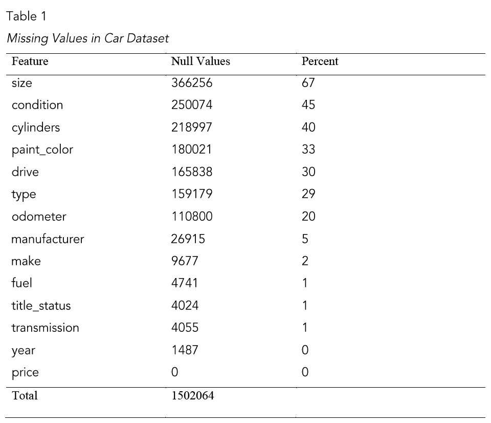
Data cleaning: First step for data cleaning was to remove unnecessary features. For this purpose, ‘url’,’image_url’, ‘lat’, ‘long’, ‘city_url’, ‘desc’, ‘city’, ‘VIN’ features were dropped totally. As a next step, it was investigated number of null points and percentage of null data points for that feature (Table 1).
As a next step, extreme values were dropped because they inhibit prediction power of the model. Firstly, cars that had listed as more than $100.000 were dropped. There were only 580 out of 550313 data points that has over 100k price value. It addresses only small percentage of buyers. In addition, there were 61726 cars that has a price lower than $750. These values were also dropped from data-set because these prices are noise for the data. Secondly, cars that have odometer value over 300.000 miles and lower than 10 miles were dropped. And lastly, cars from earlier than 1985 were dropped. For our analysis, these data points can be considered as outliers.
As the second step, some missing values were filled with appropriate values. For the missing ‘condition’ values, it was paid attention to fill depending on category. Average odometer of all ‘condition’ sub-categories were calculated. Then, missing values were filled by considering this average odometer values for each condition sub-category. In addition, cars that have model value higher than 2019 were filled as ‘new’, and between 2017–2019 were filled as ‘like new’. At the end of this process, all missing values in ‘condition’ feature were cleaned.
Others were filled as by using ‘ffill’ method. This method propagates last valid observation forward to next valid. Thus, the last known value is available at every time point. Up to now, all missing values at odometer, condition, condition and price features were clear. After this step, all data became clean. After this operation, there were 380,962 observations in the data that will be studies and analyzed.

The Exploratory Data Analysis (EDA)
While exploring the data, we will look at the different combinations of features with the help of visuals. This will help us to understand our data better and give us some clue about pattern in data.
An examination of price trend
Price is the feature that we are predicting in this study. Before applying any models, taking a look at price data may give us some ideas.
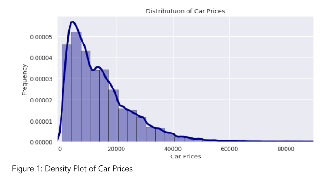
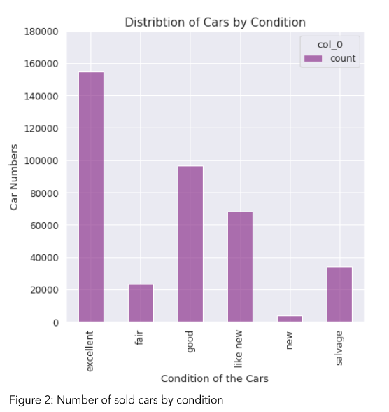
By looking at Figure 1, it can be observed that most of the used cars are less than $20,000. In addition, we see that there are still considerable number of cars that is over $20k price. We can guess that all type of cars can be cheap or expensive. But, still excellent, like new, and good condition cars are the most popular cars in used car market (Figure 2). Salvage cars are following these three categories in popularity. Therefore, it is hard to make a strong estimate of a price of a car just by considering the type or condition of a car. But we can tell it certain condition cars are popular and higher chance to be sold.
Popular features of used cars
When buying a used car, people pay serious attention to the odometer value on the car. We can see that odometer changes the price of a car significantly (Figure 3). On the other hand, this does not mean that only low odometer cars are sold. Depending on the price, high odometer cars also have buyers (Figure 4). Furthermore, most popular used cars are the ones that has odometer around 100k. Until 150k odometer, there are many cars on the market.

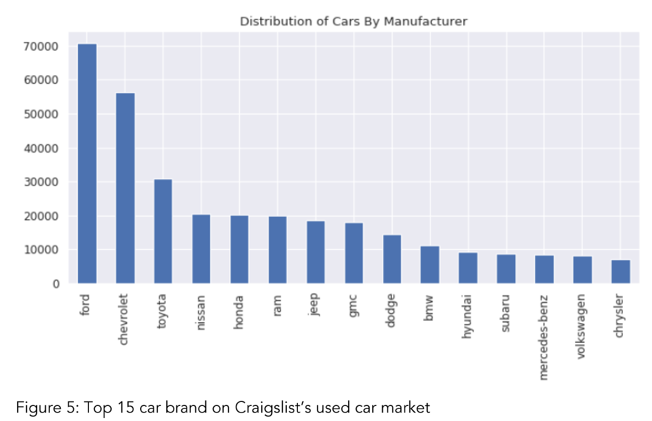
Manufacturer of a car is another important variable on used car market. Ford and Chevrolet are one dominant manufacturer in North America (Figure 5). Toyota and Nissan follow the order as big manufacturers. It can be concluded that Japanese cars have a considerable share in used car market. However, American cars are still on demand and dominant.

Transmission: Transmission is another feature that has a dominant sub category in the used car market. According to Figure 6, automatic transmission has a strong effect on people’s preference on car. In Figure 6, it can be seen that after 2000, automatic transmission cars are in the increase. In 2009, it decreases. Global economic recession might have an impact on used car market and affect market. Another interesting trend is that after 2009, other transmission is on the increase. Its market share is still so low compared to automatic transmission, but it is still considerable. The increase in other transmission type can be caused by a couple reason. First possibility is that increase in continuously variable transmission (CVT). CVT is more environmentally friendly and fuel efficient. There might be a promotion for this kind of technology. Another possibility is that some seller on Craigslist website did not fill transmission section of the car information. The website might directly put them in the ‘other’ category. This also explains the increase in the ‘other’ category of transmission.
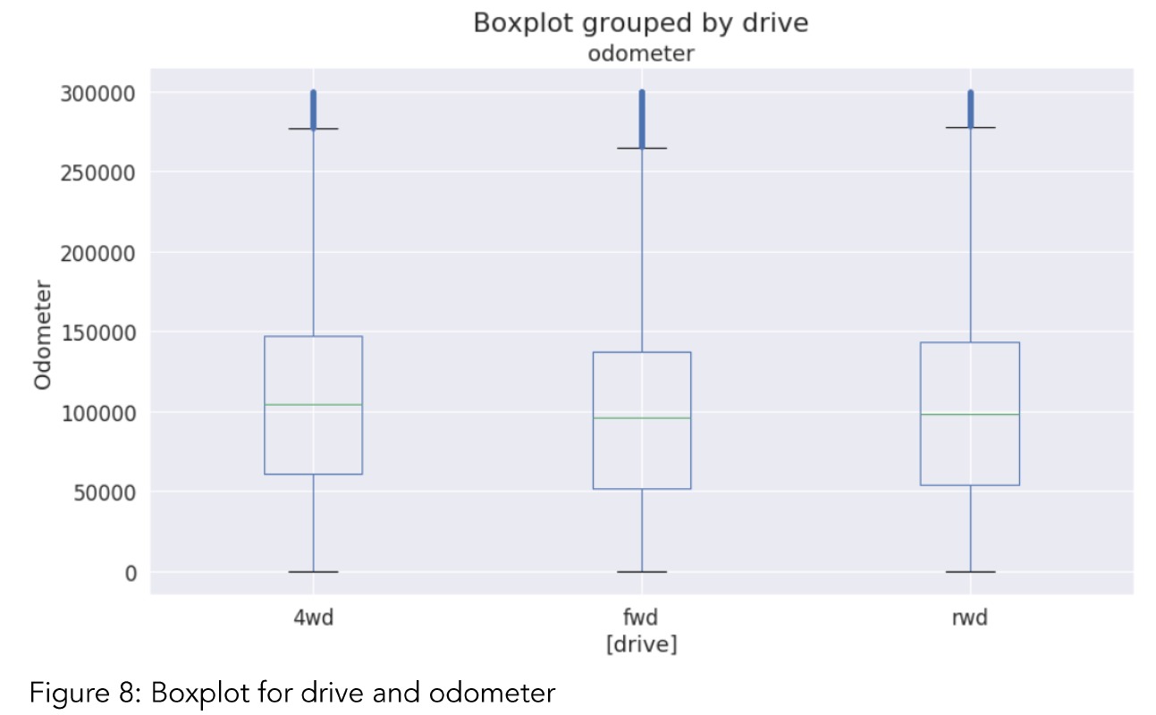
Drivetrain type: While evaluating a car, it’s important to understand what affects it’s condition. Figure 7 tells that 4wd drive cars more durable and reliable. It can be seen that 4wd cars are the most popular in terms of numbers. In the long run, they can keep their ability to run better compared to rwd and fwd drive train. 4wd has highest numbers of ‘excellent’, ‘like new’, and ‘good’ condition’ of cars. On the other hand, we need to keep in mind that compared to total number, it’s hard to say that 4wd cars higher rate of “excellent” and “like new” cars (Fig.7). In addition, by looking at table 4,

we can see that average odometers for all drivetrain types are so close to each other for all quantiles. This also tells that in the used car market, drive type may not affect with odometer of cars. But their popularity is different among drivers (Table 3 and Fig 8).

Test & Hypothesis
In order to understand what affects change in price of a used car, the relation between features available in the data sat will be examined by using inferential statistic methods. The primary assumption based on figures and tables is price must be affected by odometer and condition. There must be other features that affects price significantly. It will be investigated in the later phase of the study.
The first hypothesis:
Null Hypothesis: There is no significant relation between price and odometer of a car
Alt-Hypothesis: There is a significant relation between price and odometer.
The second hypothesis:
Null Hypothesis: There is no significant relation between price and condition of a car
Alt-Hypothesis: There is a significant relation between price and condition.
Odometer vs Price
Firstly, examine first hypothesis. Independent t-test is an appropriate method while examining the relation between two numerical variables. On the other hand, this test has some presumptions. Homogeneity of variances is one of the assumptions. In order to check whether homogeneity of variance assumption is violated or not, Levene test is applied.
Checking homogeneity of variance: The result of the Levene test:
Levene Result (statistic=335641.8310266318, p-value=0.0)
This means that homogeneity of variance is violated. In this case, we need to use Welch’s test. Welch’s t-test is a non-parametric univariate test that tests for a significant difference between the mean of two unrelated groups. It is an alternative to the independent t-test when there is a violation in the assumption of equality of variances. Therefore, it’s appropriate for this case. Here is the result of the Welch’s test:
Welch's t-test= 740.70
p-value = 0.00
Welch-Satterthwaite Degrees of Freedom= 276855.87
Here, p-value is significant. This tells that there is a significant relation between odometer and price of a car. For a reference, there is no harm to conduct an independent t-test. It can provide some ideas even though it’s not a robust method for odometer and price features.
Checking normality: For checking normality, q-q plot helps us. Figure 9 tells that there is a violation of normality. This means that the data points that are used are not distributed normally. In addition, Shapiro-Wilk test was performed for checking normality.
Result:(0.9586305022239685, 0.0)
Here, the first value is W-test statistic and the second value is the p-value. For N > 5000, the W test statistic is accurate but the p-value may not be. By considering p-value of Shapiro-Wilk test, it can be concluded that the data is not normally distributed.
In this situation, we have problem with initial data points. May be, filtering data can solve this issue. For this purpose, the values of odometer and price that are two standard deviation away from mean were dropped and independent t-test applied.

As it was stated earlier, t-test is not appropriate here because of violation of equality of variances assumption and normality assumption. On the other hand, we can still interpret the result while keeping in mind that it is not reliable. According to table 5, the correlation is 0.90. This indicates a strong relation between price and odometer. In addition, p-value is low and statistically significant. Effect size (Cohen’s d) is 4.17 which is a large value. A d of 4 indicates they differ by 4 standard deviations. This means that two groups’ means differ by 4 standard deviations or more, thus the difference is significant.

By considering these results of Welch’s test and table 5, it can be concluded that odometer and price have a significant relation. Therefore, first hypothesis’s null hypothesis is rejected. Rejecting null has some possible meanings:
- Alternative hypothesis is true.
- There can be type 2 error which implies that null hypothesis is rejected mistakenly
- Yes, there is a statistical significance. But it does not imply practical significance.
Condition vs Price
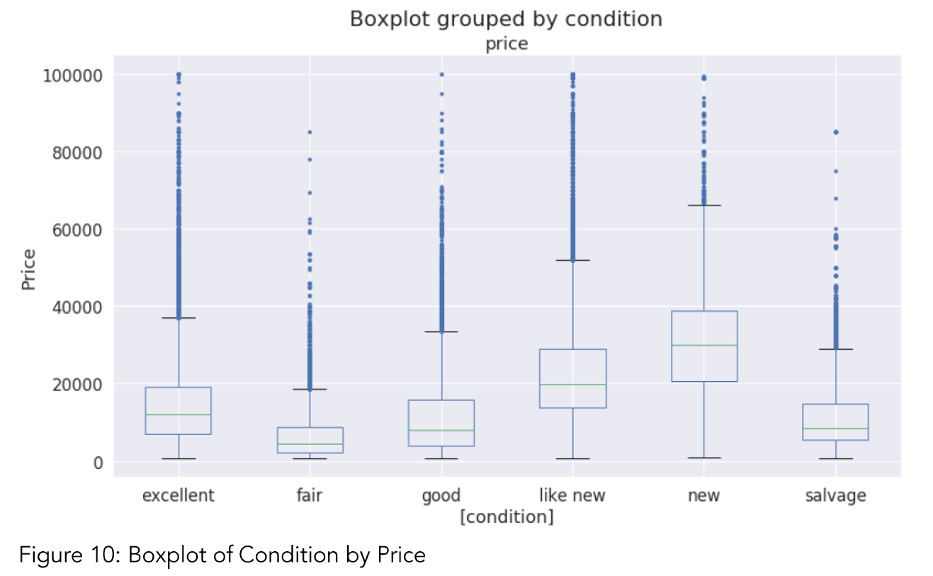
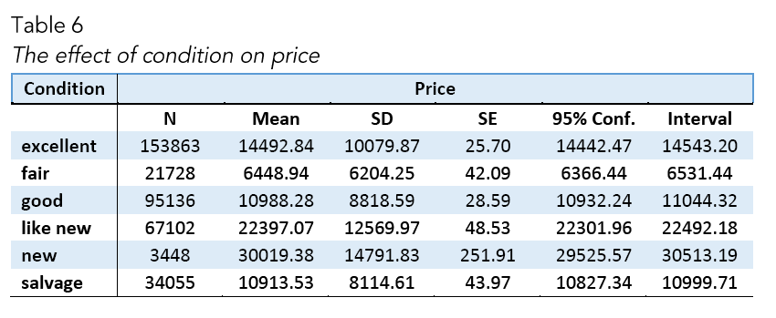
The second hypothesis of this study focuses on effect of a car’s condition on its price. In order to understand this relation, Table 6 and Figure 6 can be useful. By looking at Figure 10, it can be said that ‘condition’ effects median price of cars seriously. On the other hand, there are a lot of outliers in the condition values which is an expected result for such a lar dataset. We do not see outliers at the bottom of the Figure 10. This is mostly because during data cleaning, cars that lower than $750 price were dropped.
Now, it is time to check the relation between condition and price. Before applying any linear relation test, diagnostic tests must be applied. Hence, it can be checked whether the relation satisfies the four assumptions: Linearity of residuals, Independence of residuals, Normal distribution of residuals, Equal variance of residuals. In order to test normality Jarque-Bera were conducted, for checking equal variance of residuals Omnibus test were applied. In addition, for checking multicollinearity Condition Number (condno) test were used, and to detect the presence of autocorrelation The Durban-Watson test were applied (Table 7).

By considering Table 7, Jarque-Bera p-value and Omni p-value are significant. This indicates that there is a violation of normality and homogeneity of variance. In addition, The Durbin Watson (DW) statistic is a test for autocorrelation in the residuals from a statistical regression analysis. The Durbin-Watson statistic will always have a value between 0 and 4. A value of 2.0 means that there is no autocorrelation detected in the sample. Values from 0 to less than 2 indicate positive autocorrelation and values from from 2 to 4 indicate negative autocorrelation. The Durbin Watson score of ‘condition’ and ‘price’ is 1,49 which indicates that it’s a weak but positive correlation.
Inference of the results for ‘condition’
The hypothesis was:
H0: There is no significant relation between price and condition of a car
By considering test result, we fail to reject null hypothesis. However, the hypothesis is based on a linear relation. Therefore, there are some possible interpretations for this situation:
· There can be a relation between ‘condition’ and ‘price’ but it is not a linear relation. It can be a non-linear relation.
· There can be a linear relation but our data may not be representative and failed us to see the relation.
· The null hypothesis is correct and there is no a significant relation between ‘condition’ and ‘price’.
Challenges of Inferential Statistics
In this data set, one of the biggest challenges is that the distribution of the predictor variables was violation normality. That’s why, classical statistical methods were not much helpful for analyzing this data. Besides, in the dataset there are only 3 numerical variables among 14 variables. This limits our opportunity to use Pearson-r correlation.
Therefore, we will move on the next section. In the next section, machine learning models will be applied and performance of the models will be tested by using mean absolute error (MAE), mean squared error (MSE) and root mean squared error (RMSE).
Machine Learning Models
This section used applied machine learning models as a framework for the data analysis. The data set is a supervised data which refers to fitting a model of dependent variables to the independent variables, with the goal of accurately predicting the dependent variable for future observations or understanding the relationship between the variables (Gareth, Daniela, Trevor, & Tibshirani, 2013). In relation to the data set, literature suggests below listed methods can be appropriate.
In this section, these machine learning models will be applied in order:
· Random Forest
· Ridge Regression
· Lasso
· K-Nearest Neighbor
· XGBoost
In addition, before ridge regression, simple linear model will be applied and results will be considered.
Pre-processing the data
Label Encoding. In the dataset, there are 13 predictors. 2 of them are numerical variables while rest of them are categorical. In order to apply machine learning models, we need numeric representation of the features. Therefore, all non-numeric features were transformed into numerical form.
Train the data. In this process, 20% of the data was split for the test data and 80% of the data was taken as train data.
Scaling the Data. While exploring the data in the previous sections, it was seen that the data is not normally distributed. Without scaling, the machine learning models will try to disregard coefficients of features that has low values because their impact will be so small compared to the big value features.
While scaling, it’s also important to scale with correct method because inappropriate scaling causes inappropriate target quantification and inappropriate measures of performance (Hurwitz, E., & Marwala, 2012). Min-max scaler is appropriate especially when the data is not normal distribution and want outliers to have reduced influence. Besides, both ridge and lasso get influenced by magnitude of the features to perform regularization. Therefore, Min-Max Scaler was used on the dataset.
Random Forest
Random forest is a set of multiple decision trees. Deep decision trees may suffer from overfitting, but random forest prevents overfitting by creating trees on random subsets. That’s why, it’s a good model to in the analysis.
In the analysis, 200 trees were created. In general, the more trees give the better results. As a result, 4001.8 RMSE and 2122.92 mean absolute error (MAE) obtained (Table 8).

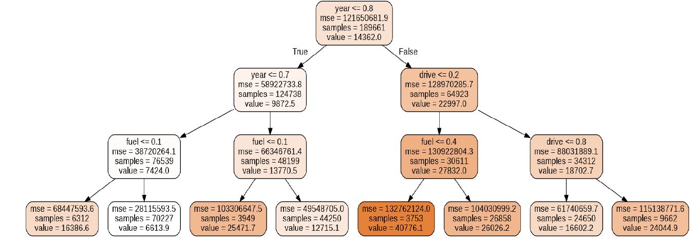
If we look at Figure 11, we see that there are seven leaf nodes. This tree uses only three variables: year, drive and fuel. The leaf nodes do not have a question because these are where the final predictions are made. To classify a new point, simply move down the tree, using the features of the point to answer the questions until you arrive at a leaf node where the class is the prediction.
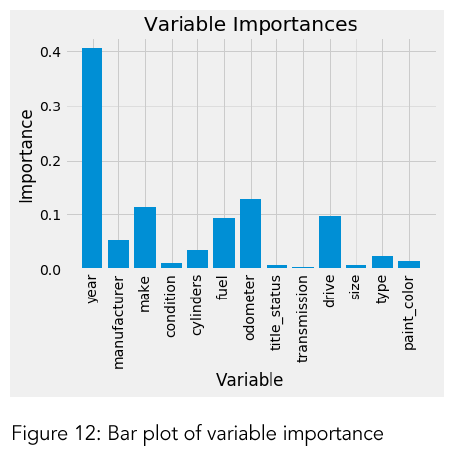
Variable Importance: In order to quantify the usefulness of all the variables in the entire random forest, we can look at the relative importance of the variables. Figure 12 is a simple bar plot of the feature importance to illustrate the disparities in the relative significance of the variables. For this study, reaching 90% of the cumulative importance is considered as a success.
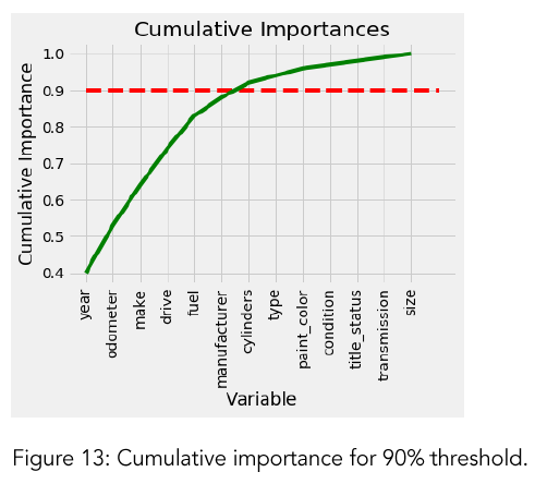
Model with only important features: Number of features for 90% cumulative importance is 7 (Fig. 13). The features are: year, odometer, make, drive, fuel, manufacturer, cylinders. The ultimate purpose of the modelling is to get a smaller number of features that can give us a strong prediction. At this point, the model was run with only these seven important features. The new RMSE is 3960.11 (Table 9). This score is slightly better than the full model (4001.80 % vs 3960.11). In addition, this performance was obtained just by using 7 features instead of 13. Therefore, it can be considered as an improvement in both prediction power and computational cost.

Linear Regression
Before applying ridge and lasso, examining linear regression results can be useful (Table 10).

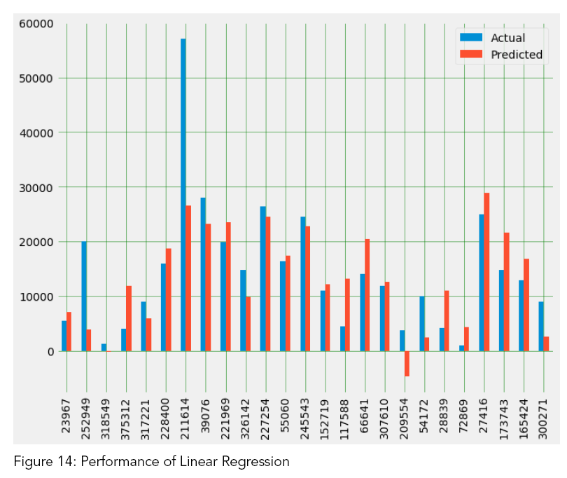
As we can see in the Table 10, the performance of the linear regression is not much good compared to random forest. The difference between actual values and predicted values is worthy of notice (Fig. 14). That’s why, we need different models that may give better predictions results.
Ridge Regression
Ordinary least square (OLS) gives unbiased regression coefficients (maximum likelihood estimates “as observed in the data-set”). Ridge regression and lasso allow to regularize (“shrink”) coefficients. In Figure 15, it can be seen how coefficients are shringking with increasing value of alpha.

In order to find best alpha value in ridge regression, cross validation was applied. The results are presented at table 11.

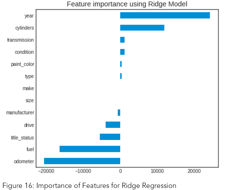
Compared to OLS, the performance of ridge is almost same. Considering figure 16, ridge regression suggest that these six variables are the most important ones: year, odometer, fuel, cylinders, title status and drive.
Lasso
Ridge shrinks the coefficients of the variables but does not make them zero. This may be good for certain cases, but it can create a challenge in model interpretation in settings in which the number of variables is quite large (Gareth, Daniela, Trevor, & Tibshirani, 2013). For this dataset, number of variables is not large, so there is no a serious need for lasso model. However, taking a look at lasso can give us another perspective. And, there is no harm to applying lasso to the dataset other than investing time and effort.
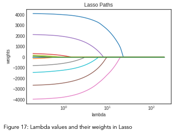
In order to find best lambda value from Fig. 17, cross-validation was applied. In this evaluation, obtained RMSE is 7578.82 (table 12).

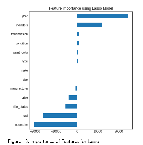
Similar to the ridge results, lasso also gave six significant features: year, odometer, fuel, cylinders, title status, drive. While making final interpretation, this can be taken into consideration.
K-nearest Neighbors (KNN)
KNN-classifier can be used when your data set is small enough, so that KNN-Classifier completes running in a shorter time. The KNN algorithm can compete with the most accurate models because it makes highly accurate predictions. Therefore, we can use the KNN algorithm for applications that require a good prediction but do not require a human-readable model. The quality of the predictions depends on the distance measure. Therefore, the KNN algorithm is suitable for applications for which sufficient domain knowledge is available (IBM Knowledge Center, n.d.) Because we have 13 features for prediction, KNN is an appropriate method to apply for this study. For evaluation of the RMSE values, we can take a look at table 12.

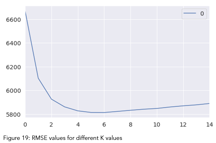
At table 13 and fig. 19, it can be observed that RMSE value is at lowest when k is seven. On the other hand, there is no significant difference between RMSE values for k are two and seven. The rationale here is that if a set of K values appear to be more or less equally good, then we might as well choose the simplest model — that is, the model with the smallest number of predictors. For our case, we can justify to choose 2 predictors because it has lowest RMSE value (Table 13). However, considering previous models, six or seven predictors still have a strong reason to choose and more consistent with them.
XGBoost
XGBoost is a specific implementation of the Gradient Boosting method which uses more accurate approximations to find the best tree model. It employs a number of nifty tricks that make it exceptionally successful, particularly with structured data. XGBoost has additional advantages: training is very fast and can be parallelized / distributed across clusters. Therefore, XGBoost was another model that is used in this study. Performance of XGBoost is as shown in Table (table 14).
Fitting the model: As a first step, the objective parameter is set to be linear.
For the next step, 3-fold cross validation was performed. Max depth was chosen as 3. So that the model was kept simple. Finally, the number of times is set to perform boosting as 50.

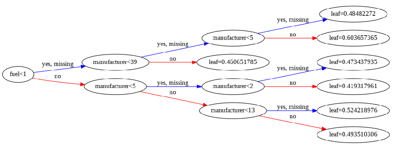
Figure 20 provides a different perspective to the model. The final prediction for a given value (leaf) is the sum of predictions from each branch. On the other hand, decision tree may not be a robustness way for making prediction for our data set because it tries to make a regression but the dataset has many categorical variables. In addition to decision tree, feature importance figure (fig. 21) can give another perspective for evaluation. By considering figure 21, it can be said that odometer, manufacturer, year, and make are important features to include the model.

Conclusion
By performing different models, it was aimed to get different perspectives and eventually compared their performance. With this study, it purpose was to predict prices of used cars by using a dataset that has 13 predictors and 380962 observations. With the help of the data visualizations and exploratory data analysis, the dataset was uncovered and features were explored deeply. The relation between features were examined. At the last stage, predictive models were applied to predict price of cars in an order: random forest, linear regression, ridge regression, lasso, KNN, XGBoost.
By considering all four metrics from table 15, it can be concluded that random forest the best model for the prediction for used car prices. Random Forest as a regression model gave the best MAE, MSE and RMSE values (Table 14). According to random forest, here are the most important features: year, odometer, make, drive, fuel, manufacturer, cylinders. These features provide 3960.11 RMSE just by using seven listed features.

Limitations of the Study and Suggestion for Further Studies
This study used different models in order to predict used car prices. However, there was a relatively small dataset for making a strong inference because number of observations was only 380962. Gathering more data can yield more robust predictions. Secondly, there could be more features that can be good predictors. For example, here are some variables that might improve the model: number of doors, gas/mile (per gallon), color, mechanical and cosmetic reconditioning time, used-to-new ratio, appraisal-to-trade ratio.
Another point that that has room to improvement is that data cleaning process can be dome more rigorously with the help of more technical information. For example, instead of using ‘ffill’ method, there might be indicators that helps to fill missing values more meaningfully.
As suggestion for further studies, while pre-processing data, instead of using label encoder, one hot encoder method can be used. Thus, all non-numeric features can be converted to nominal data instead of ordinal data (Raschka & Mirjalili, 2017). This may cause a serious change in performance of predictive models. Also, after training the data, instead of min-max scaler, standard scaler can be performned and results can be compared. Different scalers can be checked whether there is an improvement in prediction power of models or not.
Suggest:
☞ Machine Learning Zero to Hero - Learn Machine Learning from scratch
☞ Introduction to Machine Learning with TensorFlow.js
☞ Platform for Complete Machine Learning Lifecycle
☞ Python Machine Learning Tutorial (Data Science)
☞ Free resources to learn Machine Learning 🔥 || How to learn Machine Learning for free in 2021